Thresholding method for imbalanced classification
Introduction
Thresholding is a simple method that can improve the accuracy of a classifier in the case when it was trained on an imbalanced dataset. It relies on Bayes’ Theorem and the fact that neural networks estimate posterior distribution (Richard & Lippmann, 1991). In practice, it means that given a datapoint $x$, the output for a neuron representing class $i$ corresponds to
\[y_i(x) = p(i|x) = \frac{p(i) \cdot p(x|i)}{p(x)}\]where $p(i)$ is a prior probability for class $i$.
In a standard case, equal priors are assumed for all classes. However, it is not always the case. E.g. in medical datasets some diseases are known to have a prevalence of less than 1%.
A class prior can be estimated based on the number of examples in a training set unless we have a good reason to think that our training set is not reflective of the true class distribution. Otherwise, for class $i$ we have:
\[p(i) = \frac{|i|}{\sum_{k}{|k|}}\]where $|i|$ denotes the number of unique examples in class $i$.
Finally, the adjusted network output for class $i$ can be obtained by dividing the original output by the corresponding prior.
Simple example
Let us assume that we have already trained a classifier on a training set with the number of examples per class as following:
\[[100, 400, 500]\]Then, we tested our model on a test case $x$ and it returned the vector of class probabilities:
\[y = [0.2, 0.2, 0.6]\]In this case, the predicted class would be:
\[argmax(y) = 2\]Now, to apply thresholding method, we have to compute the vector of priors. In this case, it will be:
\[p = [100/1000, 400/1000, 500/1000] = [0.1, 0.4, 0.5]\]And adjusted predictions are obtained by dividing original predictions element-wise by the vector of priors:
\[y' = y \oslash p = [\frac{0.2}{0.1}, \frac{0.2}{0.4}, \frac{0.6}{0.5}] = [2.0, 0.5, 1.2]\]The predicted class has now changed to:
\[argmax(y') = 0\]Python implementation
For impatient readers, the full notebook is available as a GitHub gist.
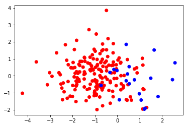
First, let us build a simple dataset based on two Gaussian distributions.
# 20 positive and 180 negative training examples
X1_train = np.random.normal((1.0, 0.0), 1.0, (20, 2))
X0_train = np.random.normal((-1.0, 0.0), 1.0, (180, 2))

X_train = np.vstack((X0_train, X1_train))
y_train = np.array(180 * [0] + 20 * [1])

X1_test = np.random.normal((1.0, 0.0), 1.0, (500, 2))
X0_test = np.random.normal((-1.0, 0.0), 1.0, (500, 2))

X_test = np.vstack((X0_test, X1_test))
y_test = np.array(500 * [0] + 500 * [1])
The training set looks like this:
We will use it to train a simple neural network with 2 hidden units:
nn = MLPClassifier(solver='lbfgs', hidden_layer_sizes=(2), activation='logistic', random_state=42)
nn.fit(X_train, y_train)
The decision boundary looks like reasonably discriminating positive (blue) and negative (red) examples:
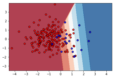
The accuracy evaluated on the test set is:
"Accuracy = {}%".format(100 * nn.score(X_test, y_test))
Accuracy = 75.1%
We will attempt to improve it using thresholding method. To do that, we need to implement functions to estimate class priors and generate adjusted predictions.
def priors(y):
    return np.unique(y, return_counts=True)[1] / float(len(y))
def predict_thresholded(nn, X, p):
    y_pred = nn.predict_proba(X)
    y_pred_th = y_pred / p
    return np.argmax(y_pred_th, axis=1)
Now, we can use them and evaluate the performance again:
p = priors(y_train)
y_pred_test = predict_thresholded(nn, X_test, p)
"Accuracy = {}%".format(100 * accuracy_score(y_test, y_pred_test))
Accuracy = 84.2%
We were able to improve the accuracy by over 9%. However, the thresholding method only scales the outputs by multiplying them by a constant number. It must be noted that the discriminative power of a classifier (e.g. as measured using ROC) does not change in this case.
Links
- Code: GitHub gist
- Class imbalance: arXiv:1710.05381
- Extended report: diva2:1165840